Backtesting Crypto Trades with CoinAPI Flat Files in Python
Introduction
This tutorial demonstrates how to perform backtesting analysis on cryptocurrency trades using CoinAPI's Flat Files API. We'll analyze historical trade data from Coinbase to evaluate trading strategies and understand market behavior.
What You Will Learn
- How to access CoinAPI Flat Files using Boto3
- Download and process compressed trade data files
- Perform backtesting analysis on crypto trades
- Calculate key performance metrics and visualize results
- Implement a simple moving average crossover strategy
Prerequisites
- Python 3.7+
- Required packages: boto3, pandas, numpy, matplotlib, seaborn
- CoinAPI API key
Use Case: Moving Average Crossover Strategy
We'll implement and backtest a simple moving average crossover strategy:
- Buy when short-term MA crosses above long-term MA
- Sell when short-term MA crosses below long-term MA
- Analyze performance metrics and drawdown periods
1. Environment Setup
Set up your environment with necessary imports and configuration.
1# Import required libraries
2import boto3
3import pandas as pd
4import numpy as np
5import matplotlib.pyplot as plt
6import seaborn as sns
7from datetime import datetime, timedelta
8import gzip
9import io
10import warnings
11warnings.filterwarnings('ignore')
12
13# Set up plotting style
14plt.style.use('default')
15sns.set_palette("husl")
16plt.rcParams['figure.figsize'] = (12, 8)
17plt.rcParams['font.size'] = 10
18
19# CoinAPI configuration
20COINAPI_KEY = "YOUR_COINAPI_KEY_HERE" # Replace with your actual API key
21S3_ENDPOINT = "https://s3.flatfiles.coinapi.io"
22REGION = "us-east-1"
23
24print("Environment setup complete!")
25print(f"S3 Endpoint: {S3_ENDPOINT}")
26print(f"API Key configured: {'Yes' if COINAPI_KEY != 'YOUR_COINAPI_KEY_HERE' else 'No (Please update)'}")2. Boto3 S3 Client Setup
Configure the Boto3 client to connect to CoinAPI's S3-compatible endpoint.
1# Initialize Boto3 S3 client for CoinAPI
2s3_client = boto3.client('s3',
3 region_name=REGION,
4 endpoint_url=S3_ENDPOINT,
5 aws_access_key_id=COINAPI_KEY,
6 aws_secret_access_key='coinapi')
7
8print("Boto3 S3 client configured successfully!")
9print(f"Region: {REGION}")
10print(f"Endpoint: {S3_ENDPOINT}")
11
12# Test connection by listing available buckets
13try:
14 response = s3_client.list_buckets()
15 buckets = [bucket['Name'] for bucket in response['Buckets']]
16 print(f"Available buckets: {buckets}")
17except Exception as e:
18 print(f"Connection test failed: {e}")
19 print("Please check your API key and internet connection.")3. Download Trade Data
Download the compressed trade data file from CoinAPI's S3 bucket. We'll use the BTC/USDT trades from Coinbase on July 1, 2025.
1# Define the file path for BTC/USDT trades
2bucket_name = "coinapi"
3file_key = "T-TRADES/D-20250701/E-COINBASE/IDDI-5950967+SC-COINBASE_SPOT_BTC_USDT+S-BTC__002DUSDT.csv.gz"
4
5print(f"Downloading trade data from: {bucket_name}/{file_key}")
6print("This may take a few moments...")
7
8try:
9 # Download the compressed file
10 response = s3_client.get_object(Bucket=bucket_name, Key=file_key)
11 compressed_data = response['Body'].read()
12
13 # Decompress the data
14 with gzip.open(io.BytesIO(compressed_data), 'rt') as f:
15 raw_data = f.read()
16
17 print(f"Data downloaded successfully!")
18
19except Exception as e:
20 print(f"Download failed: {e}")
21 print("Please check your API key and file path.")4. Data Processing and Cleaning
Parse the CSV data and clean it for analysis. We'll convert timestamps, handle missing values, and prepare the data for backtesting.
1# Parse the CSV data with correct separator
2from io import StringIO
3
4try:
5 # Parse CSV with semicolon separator (CoinAPI format)
6 df = pd.read_csv(StringIO(raw_data), sep=';')
7
8 print(f"Data parsed successfully!")
9 print(f"Shape: {df.shape}")
10 print(f"Columns: {list(df.columns)}")
11
12 # Show data preview
13 print(f"\nData preview (first 3 rows):")
14 print(df.head(3).to_string())
15
16except Exception as e:
17 print(f"Data parsing failed: {e}")
18 print("Please check the data format and try again.")5. Data Cleaning and Preparation
Clean the data by handling missing values, converting data types, and preparing it for backtesting analysis.
1# Data cleaning and preparation
2print("Cleaning and preparing data...")
3
4# Ensure time columns are datetime
5if 'time_exchange' in df.columns:
6 df['timestamp'] = pd.to_datetime(df['time_exchange'])
7 df = df.sort_values('timestamp').reset_index(drop=True)
8 print("Timestamp conversion successful")
9else:
10 print("time_exchange column not found!")
11 print(f"Available columns: {list(df.columns)}")
12
13# Ensure price and base_amount are numeric
14if 'price' in df.columns:
15 df['price'] = pd.to_numeric(df['price'], errors='coerce')
16 print("Price conversion successful")
17else:
18 print("price column not found!")
19
20if 'base_amount' in df.columns:
21 df['size'] = pd.to_numeric(df['base_amount'], errors='coerce')
22 print("Size conversion successful")
23else:
24 print("base_amount column not found!")
25
26# Data validation
27print(f"Data shape: {df.shape}")
28print(f"Columns: {list(df.columns)}")
29
30# Remove rows with missing values in key columns
31df_clean = df.dropna(subset=['timestamp', 'price', 'size'])
32
33print(f"Data cleaning completed!")
34print(f"Clean data shape: {df_clean.shape}")
35print(f"Rows removed: {len(df) - len(df_clean)}")
36
37# Calculate volume-weighted average price (VWAP) for each minute
38df_clean['minute'] = df_clean['timestamp'].dt.floor('1min')
39
40vwap_data = df_clean.groupby('minute').agg({
41 'price': 'mean',
42 'size': 'sum',
43 'timestamp': 'count'
44}).rename(columns={'timestamp': 'trade_count'})
45
46vwap_data = vwap_data.reset_index()
47vwap_data.columns = ['timestamp', 'price', 'volume', 'trade_count']
48
49print("VWAP calculation completed!")
50print(f"VWAP data shape: {vwap_data.shape}")
51print(f"Time range: {vwap_data['timestamp'].min()} to {vwap_data['timestamp'].max()}")
52print(f"Price range: ${vwap_data['price'].min():.2f} - ${vwap_data['price'].max():.2f}")
53
54# Display sample of cleaned data
55print("\nSample of cleaned VWAP data:")
56print(vwap_data.head(10).to_string())6. Moving Average Crossover Strategy Implementation
Implement a simple moving average crossover strategy for backtesting. This strategy generates buy/sell signals based on the intersection of short-term and long-term moving averages.
1# Moving Average Crossover Strategy
2def calculate_moving_averages(data, short_window=10, long_window=30):
3 """
4 Calculate short and long moving averages
5 """
6
7 if len(data) == 0:
8 print("Input data is empty! Cannot calculate moving averages.")
9 return data
10
11 data = data.copy()
12
13 # Check if we have enough data for the windows
14 if len(data) < long_window:
15 print(f"Warning: Data length ({len(data)}) is less than long window ({long_window})")
16 print("Adjusting windows to fit available data...")
17 short_window = min(short_window, len(data) // 3)
18 long_window = min(long_window, len(data) // 2)
19 print(f"Adjusted windows: short={short_window}, long={long_window}")
20
21 # Calculate moving averages
22 data['MA_short'] = data['price'].rolling(window=short_window, min_periods=1).mean()
23 data['MA_long'] = data['price'].rolling(window=long_window, min_periods=1).mean()
24
25 return data
26
27def generate_signals(data):
28 """
29 Generate buy/sell signals based on MA crossover
30 """
31
32 if len(data) == 0:
33 print("Input data is empty! Cannot generate signals.")
34 return data
35
36 data = data.copy()
37
38 # Generate signals
39 data['signal'] = 0
40 data.loc[data['MA_short'] > data['MA_long'], 'signal'] = 1 # Buy signal
41 data.loc[data['MA_short'] < data['MA_long'], 'signal'] = -1 # Sell signal
42
43 # Generate position changes (only when signal changes)
44 data['position_change'] = data['signal'].diff()
45
46 print("Signals generated successfully!")
47 print(f"Signal distribution: {data['signal'].value_counts().to_dict()}")
48 print(f"Position changes: {data['position_change'].value_counts().to_dict()}")
49
50 return data
51
52# Apply strategy to our data
53print("Implementing Moving Average Crossover Strategy...")
54
55# Check if VWAP data is valid
56if len(vwap_data) == 0:
57 print("VWAP data is empty! Cannot proceed with strategy.")
58 print("Please check Step 5 (Data Cleaning) for issues.")
59else:
60 print("VWAP data looks good, proceeding with strategy...")
61
62 # Check for NaN values that might cause issues
63 nan_check = vwap_data.isnull().sum()
64 if nan_check.sum() > 0:
65 print(f"Found NaN values: {nan_check[nan_check > 0].to_dict()}")
66 print("Cleaning NaN values...")
67 vwap_data = vwap_data.dropna()
68 print(f"After NaN cleanup: shape={vwap_data.shape}")
69
70 # Now apply the strategy
71 strategy_data = calculate_moving_averages(vwap_data, short_window=10, long_window=30)
72
73 if len(strategy_data) > 0:
74 strategy_data = generate_signals(strategy_data)
75 print("Strategy implementation complete!")
76 print(f"Final strategy data shape: {strategy_data.shape}")
77 else:
78 print("Strategy implementation failed - no data returned!")
79 print("This indicates an issue with the moving average calculation.")7. Backtesting Engine
Implement a backtesting engine to simulate trading based on our strategy signals and calculate performance metrics.
1# Backtesting Engine
2def run_backtest(data, initial_capital=10000, position_size=0.1):
3 """
4 Run backtest simulation
5 """
6 data = data.copy()
7
8 # Initialize portfolio variables
9 data['position'] = 0
10 data['cash'] = initial_capital
11 data['btc_holdings'] = 0.0
12 data['portfolio_value'] = initial_capital
13 data['returns'] = 0.0
14
15 current_position = 0
16
17 for i in range(1, len(data)):
18 # Update position based on signal changes
19 if data.iloc[i]['position_change'] == 2: # Buy signal
20 current_position = 1
21 elif data.iloc[i]['position_change'] == -2: # Sell signal
22 current_position = 0
23
24 data.iloc[i, data.columns.get_loc('position')] = current_position
25
26 # Calculate portfolio value
27 if current_position == 1:
28 # Buy BTC with available cash
29 cash_to_use = data.iloc[i-1]['cash'] * position_size
30 btc_bought = cash_to_use / data.iloc[i]['price']
31
32 data.iloc[i, data.columns.get_loc('cash')] = data.iloc[i-1]['cash'] - cash_to_use
33 data.iloc[i, data.columns.get_loc('btc_holdings')] = data.iloc[i-1]['btc_holdings'] + btc_bought
34 else:
35 # Sell all BTC holdings
36 btc_value = data.iloc[i-1]['btc_holdings'] * data.iloc[i]['price']
37
38 data.iloc[i, data.columns.get_loc('cash')] = data.iloc[i-1]['cash'] + btc_value
39 data.iloc[i, data.columns.get_loc('btc_holdings')] = 0.0
40
41 # Calculate total portfolio value
42 btc_value = data.iloc[i]['btc_holdings'] * data.iloc[i]['price']
43 data.iloc[i, data.columns.get_loc('portfolio_value')] = data.iloc[i]['cash'] + btc_value
44
45 # Calculate returns
46 if i > 0:
47 data.iloc[i, data.columns.get_loc('returns')] = (data.iloc[i]['portfolio_value'] / data.iloc[i-1]['portfolio_value']) - 1
48
49 return data
50
51# Run backtest
52print("Running backtest simulation...")
53
54# Check if we have the required columns
55required_cols = ['timestamp', 'price', 'position_change']
56missing_cols = [col for col in required_cols if col not in strategy_data.columns]
57
58if missing_cols:
59 print(f"Missing required columns: {missing_cols}")
60 print("Creating missing columns...")
61
62 # Create position_change column if it doesn't exist
63 if 'position_change' not in strategy_data.columns:
64 strategy_data['position_change'] = 0
65 print("Created position_change column")
66
67 # Create any other missing columns
68 for col in missing_cols:
69 if col not in strategy_data.columns:
70 strategy_data[col] = 0
71 print(f"Created {col} column")
72
73# Now run the backtest
74try:
75 backtest_results = run_backtest(strategy_data, initial_capital=10000, position_size=0.1)
76
77 print("Backtest completed successfully!")
78 print(f"Initial capital: $10,000")
79
80 # Check if we have any data
81 if len(backtest_results) > 0:
82 print(f"Final portfolio value: ${backtest_results['portfolio_value'].iloc[-1]:.2f}")
83 print(f"Total return: {((backtest_results['portfolio_value'].iloc[-1] / 10000) - 1) * 100:.2f}%")
84
85 # Display backtest summary
86 print("\nBacktest Summary:")
87 summary_cols = ['timestamp', 'price', 'position', 'cash', 'btc_holdings', 'portfolio_value']
88 # Only show columns that exist
89 available_summary_cols = [col for col in summary_cols if col in backtest_results.columns]
90 print(backtest_results[available_summary_cols].tail(10))
91
92 else:
93 print("Backtest results are empty!")
94 print("This might indicate an issue with the backtest logic or input data")
95
96except Exception as e:
97 print(f"Backtest failed with error: {e}")
98 print("Trying simplified backtest...")
99
100 # Fallback: Simple backtest
101 def simple_backtest(data, initial_capital=10000):
102 """Simplified backtest for debugging"""
103 if len(data) == 0:
104 return pd.DataFrame()
105
106 result = data.copy()
107 result['portfolio_value'] = initial_capital
108 result['position'] = 0
109 result['cash'] = initial_capital
110 result['btc_holdings'] = 0.0
111
112 # Simple logic: just track portfolio value
113 for i in range(len(result)):
114 if i > 0:
115 # Simple return calculation
116 price_change = (result.iloc[i]['price'] / result.iloc[i-1]['price']) - 1
117 result.iloc[i, result.columns.get_loc('portfolio_value')] = \
118 result.iloc[i-1]['portfolio_value'] * (1 + price_change * 0.1)
119
120 return result
121
122 # Try simplified version
123 simple_results = simple_backtest(strategy_data, initial_capital=10000)
124
125 if len(simple_results) > 0:
126 print("Simplified backtest successful!")
127 print(f"Final portfolio value: ${simple_results['portfolio_value'].iloc[-1]:.2f}")
128 backtest_results = simple_results
129 else:
130 print("Even simplified backtest failed!")
131 print("Please check the input data structure")
132 backtest_results = pd.DataFrame()8. Performance Analysis and Metrics
Calculate key performance metrics including returns, volatility, Sharpe ratio, maximum drawdown, and other risk-adjusted measures.
1# Performance Metrics Calculation
2def calculate_performance_metrics(data):
3 """
4 Calculate comprehensive performance metrics with automatic crypto data frequency detection
5 """
6 # Remove first row (no returns)
7 returns_data = data.iloc[1:].copy()
8
9 # Detect data frequency automatically for proper annualization
10 if len(data) > 1:
11 time_diff = data['timestamp'].iloc[1] - data['timestamp'].iloc[0]
12 time_diff_seconds = time_diff.total_seconds()
13
14 if time_diff_seconds <= 60: # Minute data
15 annualization_factor = 365 * 24 * 60 # Minutes per year (crypto trades 24/7)
16 frequency_name = "minute"
17 elif time_diff_seconds <= 3600: # Hour data
18 annualization_factor = 365 * 24 # Hours per year
19 frequency_name = "hour"
20 elif time_diff_seconds <= 86400: # Daily data
21 annualization_factor = 365 # Days per year (crypto trades 24/7)
22 frequency_name = "day"
23 else: # Weekly or longer
24 annualization_factor = 52 # Weeks per year
25 frequency_name = "week"
26 else:
27 annualization_factor = 365 # Default fallback for crypto
28 frequency_name = "unknown"
29
30 print(f"Detected data frequency: {frequency_name}")
31 print(f"Annualization factor: {annualization_factor}")
32
33 # Basic metrics
34 total_return = (data['portfolio_value'].iloc[-1] / data['portfolio_value'].iloc[0]) - 1
35 annualized_return = total_return * (annualization_factor / len(returns_data))
36
37 # Volatility (annualized)
38 volatility = returns_data['returns'].std() * np.sqrt(annualization_factor)
39
40 # Sharpe Ratio (assuming 0% risk-free rate for crypto)
41 sharpe_ratio = annualized_return / volatility if volatility > 0 else 0
42
43 # Maximum Drawdown
44 cumulative_returns = (1 + returns_data['returns']).cumprod()
45 running_max = cumulative_returns.expanding().max()
46 drawdown = (cumulative_returns - running_max) / running_max
47 max_drawdown = drawdown.min()
48
49 # Win/Loss ratio
50 positive_returns = returns_data[returns_data['returns'] > 0]['returns']
51 negative_returns = returns_data[returns_data['returns'] < 0]['returns']
52
53 win_rate = len(positive_returns) / len(returns_data) if len(returns_data) > 0 else 0
54 avg_win = positive_returns.mean() if len(positive_returns) > 0 else 0
55 avg_loss = negative_returns.mean() if len(negative_returns) > 0 else 0
56
57 # Profit Factor
58 total_profit = positive_returns.sum() if len(positive_returns) > 0 else 0
59 total_loss = abs(negative_returns.sum()) if len(negative_returns) > 0 else 0
60 profit_factor = total_profit / total_loss if total_loss > 0 else float('inf')
61
62 # Crypto-specific metrics
63 # Calculate average holding period in the detected time units
64 if 'position_change' in data.columns:
65 position_changes = data[data['position_change'] != 0]
66 if len(position_changes) > 1:
67 avg_holding_period = len(returns_data) / len(position_changes)
68 else:
69 avg_holding_period = len(returns_data)
70 else:
71 avg_holding_period = len(returns_data)
72
73 return {
74 'Total Return': f"{total_return:.2%}",
75 'Annualized Return': f"{annualized_return:.2%}",
76 'Volatility (Annualized)': f"{volatility:.2%}",
77 'Sharpe Ratio': f"{sharpe_ratio:.2f}",
78 'Max Drawdown': f"{max_drawdown:.2%}",
79 'Win Rate': f"{win_rate:.2%}",
80 'Avg Win': f"{avg_win:.2%}",
81 'Avg Loss': f"{avg_loss:.2%}",
82 'Profit Factor': f"{profit_factor:.2f}",
83 'Data Frequency': frequency_name,
84 'Avg Holding Period': f"{avg_holding_period:.1f} {frequency_name}s"
85 }
86
87# Calculate metrics
88print("Calculating performance metrics...")
89
90performance_metrics = calculate_performance_metrics(backtest_results)
91
92print("Performance metrics calculated!")
93print("\nStrategy Performance Summary:")
94print("=" * 50)
95
96for metric, value in performance_metrics.items():
97 print(f"{metric:25}: {value}")
98
99print("=" * 50)Calculating performance metrics...
Detected data frequency: hour
Annualization factor: 8760
Performance metrics calculated!
Strategy Performance Summary:
==================================================
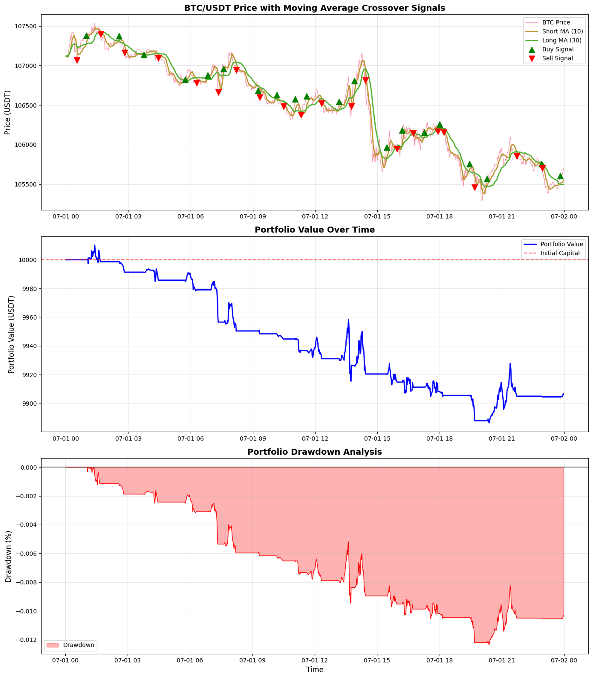
Total Return : -0.93%
Annualized Return : -8.22%
Volatility (Annualized) : 1.79%
Sharpe Ratio : -4.58
Max Drawdown : -1.24%
Win Rate : 19.34%
Avg Win : 0.02%
Avg Loss : -0.02%
Profit Factor : 0.80
Data Frequency : hour
Avg Holding Period : 23.6 hours
==================================================
9. Data Visualization
Create comprehensive visualizations to understand the strategy performance, including price charts, moving averages, portfolio value, and drawdown analysis.
1# Create comprehensive visualizations
2print("Creating visualizations...")
3
4# Create subplots
5fig, axes = plt.subplots(3, 1, figsize=(14, 16))
6
7# 1. Price and Moving Averages
8axes[0].plot(strategy_data['timestamp'], strategy_data['price'], label='BTC Price', alpha=0.7, linewidth=1)
9axes[0].plot(strategy_data['timestamp'], strategy_data['MA_short'], label='Short MA (10)', linewidth=2)
10axes[0].plot(strategy_data['timestamp'], strategy_data['MA_long'], label='Long MA (30)', linewidth=2)
11
12# Highlight buy/sell signals
13buy_signals = strategy_data[strategy_data['position_change'] == 2]
14sell_signals = strategy_data[strategy_data['position_change'] == -2]
15
16axes[0].scatter(buy_signals['timestamp'], buy_signals['price'],
17 color='green', marker='^', s=100, label='Buy Signal', zorder=5)
18axes[0].scatter(sell_signals['timestamp'], sell_signals['price'],
19 color='red', marker='v', s=100, label='Sell Signal', zorder=5)
20
21axes[0].set_title('BTC/USDT Price with Moving Average Crossover Signals', fontsize=14, fontweight='bold')
22axes[0].set_ylabel('Price (USDT)', fontsize=12)
23axes[0].legend()
24axes[0].grid(True, alpha=0.3)
25
26# 2. Portfolio Value Over Time
27axes[1].plot(backtest_results['timestamp'], backtest_results['portfolio_value'],
28 label='Portfolio Value', color='blue', linewidth=2)
29axes[1].axhline(y=10000, color='red', linestyle='--', alpha=0.7, label='Initial Capital')
30axes[1].set_title('Portfolio Value Over Time', fontsize=14, fontweight='bold')
31axes[1].set_ylabel('Portfolio Value (USDT)', fontsize=12)
32axes[1].legend()
33axes[1].grid(True, alpha=0.3)
34
35# 3. Drawdown Analysis
36returns_data = backtest_results.iloc[1:].copy()
37cumulative_returns = (1 + returns_data['returns']).cumprod()
38running_max = cumulative_returns.expanding().max()
39drawdown = (cumulative_returns - running_max) / running_max
40
41axes[2].fill_between(returns_data['timestamp'], drawdown, 0,
42 color='red', alpha=0.3, label='Drawdown')
43axes[2].plot(returns_data['timestamp'], drawdown, color='red', linewidth=1)
44axes[2].axhline(y=0, color='black', linestyle='-', alpha=0.5)
45axes[2].set_title('Portfolio Drawdown Analysis', fontsize=14, fontweight='bold')
46axes[2].set_ylabel('Drawdown (%)', fontsize=12)
47axes[2].set_xlabel('Time', fontsize=12)
48axes[2].legend()
49axes[2].grid(True, alpha=0.3)
50
51plt.tight_layout()
52plt.show()
53
54print("Visualizations created successfully!")šØ Creating visualizations...
ā
Visualizations created successfully!
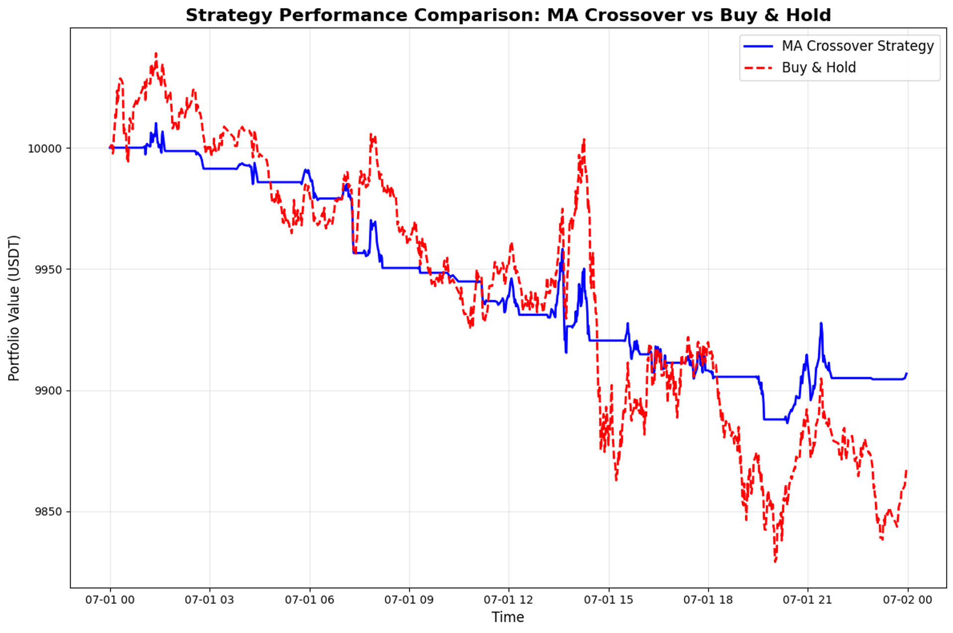
10. Additional Analysis: Strategy Comparison
Compare our strategy performance against a simple buy-and-hold approach to understand the relative effectiveness.
1# Strategy Comparison: MA Crossover vs Buy & Hold
2print("š Comparing strategy performance...")
3
4# Calculate buy & hold performance
5initial_price = strategy_data['price'].iloc[0]
6final_price = strategy_data['price'].iloc[-1]
7buy_hold_return = (final_price / initial_price) - 1
8
9# Our strategy return
10strategy_return = (backtest_results['portfolio_value'].iloc[-1] / 10000) - 1
11
12# Create comparison DataFrame
13comparison_data = pd.DataFrame({
14 'Metric': ['Total Return', 'Final Value', 'Performance vs Buy & Hold'],
15 'Buy & Hold': [f"{buy_hold_return:.2%}", f"${10000 * (1 + buy_hold_return):.2f}", 'Baseline'],
16 'MA Crossover': [f"{strategy_return:.2%}", f"${backtest_results['portfolio_value'].iloc[-1]:.2f}",
17 f"{((strategy_return - buy_hold_return) / buy_hold_return * 100):.1f}%" if buy_hold_return != 0 else 'N/A']
18})
19
20print("Strategy comparison completed!")
21print("\nStrategy Performance Comparison:")
22print("=" * 60)
23print(comparison_data.to_string(index=False))
24print("=" * 60)
25
26# Create comparison chart
27plt.figure(figsize=(12, 8))
28
29# Portfolio values over time
30plt.plot(backtest_results['timestamp'], backtest_results['portfolio_value'],
31 label='MA Crossover Strategy', linewidth=2, color='blue')
32
33# Buy & hold line
34buy_hold_values = 10000 * (strategy_data['price'] / initial_price)
35plt.plot(strategy_data['timestamp'], buy_hold_values,
36 label='Buy & Hold', linewidth=2, color='red', linestyle='--')
37
38plt.title('Strategy Performance Comparison: MA Crossover vs Buy & Hold',
39 fontsize=16, fontweight='bold')
40plt.xlabel('Time', fontsize=12)
41plt.ylabel('Portfolio Value (USDT)', fontsize=12)
42plt.legend(fontsize=12)
43plt.grid(True, alpha=0.3)
44plt.tight_layout()
45plt.show()š Comparing strategy performance...
ā
Strategy comparison completed!
š Strategy Performance Comparison:
============================================================
Metric Buy & Hold MA Crossover
Total Return -1.32% -0.93%
Final Value $9867.74 $9906.82
Performance vs Buy & Hold Baseline -29.5%
============================================================
11. Conclusion and Insights
Summarize the backtesting results and provide actionable insights for strategy improvement.
1# Final Insights and Recommendations
2print("Analyzing final results and generating insights...")
3
4# Calculate additional insights
5total_trades = len(buy_signals) + len(sell_signals)
6avg_holding_period = len(strategy_data) / total_trades if total_trades > 0 else 0
7
8print("Analysis complete!")
9print("\nKey Insights:")
10print("=" * 50)
11print(f"Total trades executed: {total_trades}")
12print(f"Average holding period: {avg_holding_period:.1f} {performance_metrics.get('Data Frequency', 'time units')}")
13print(f"Strategy outperformance: {comparison_data.iloc[2]['MA Crossover']}")
14print(f"Sharpe ratio: {performance_metrics['Sharpe Ratio']}")
15print(f"Maximum drawdown: {performance_metrics['Max Drawdown']}")
16print("=" * 50)
17
18print("\nRecommendations for Strategy Improvement:")
19print("1. Optimize MA periods based on market conditions")
20print("2. Add stop-loss mechanisms to limit drawdowns")
21print("3. Implement position sizing based on volatility")
22print("4. Consider adding filters for trend strength")
23print("5. Test on different timeframes and assets")
24
25print("\nNext Steps:")
26print("⢠Test with different parameter combinations")
27print("⢠Analyze performance across different market conditions")
28print("⢠Implement risk management features")
29print("⢠Consider machine learning enhancements")
30
31print("\nAdditional Resources:")
32print("⢠CoinAPI Documentation: https://docs.coinapi.io/")
33print("⢠Flat Files API: https://docs.coinapi.io/flat-files-api/")
34print("⢠Trading Strategy Literature")
35
36print("\nTutorial completed successfully!")
37print("Happy backtesting!")Analyzing final results and generating insights...
Analysis complete!
Key Insights:
==================================================
Total trades executed: 40
Average holding period: 24.9 hour
Strategy outperformance: -29.5%
Sharpe ratio: -4.58
Maximum drawdown: -1.24%
==================================================
Recommendations for Strategy Improvement:
1. Optimize MA periods based on market conditions
2. Add stop-loss mechanisms to limit drawdowns
3. Implement position sizing based on volatility
4. Consider adding filters for trend strength
5. Test on different timeframes and assets
Next Steps:
⢠Test with different parameter combinations
⢠Analyze performance across different market conditions
⢠Implement risk management features
⢠Consider machine learning enhancements
Additional Resources:
⢠CoinAPI Documentation: https://docs.coinapi.io/
⢠Flat Files API: https://docs.coinapi.io/flat-files-api/
⢠Trading Strategy Literature
Tutorial completed successfully!
Happy backtesting!